The Planar Euler-Savary Equation in Vectorial Notation

Stefan Gössner

Department of Mechanical Engineering, University of Applied Sciences, Dortmund, Germany.

Keywords: Euler-Savary Equation; pole transfer velocity; inflection Pole; inflection circle; rho-curves; cubic curve of stationary curvature; Ball's point; undulation point; geometric kinematics;

Abstract

The Euler-Savary Equation is discussed from a vectorial point of view. Kinematic properties of a moving link in the plane are taken to derive the inflection circle first. Then eliminating all kinematic values results in the pure geometric equation of Euler-Savary. Proceeding to the advantageous canonical coordinate system the curves of points of constant curvature, the cubic of stationary curvature and Ball's point location are derived.

Introduction

In mechanism analysis and design knowledge about direction and curvature of point paths on a moving link of kinematic chains proves itself valuable and was intensively studied in the past [1,2,3,4]. In this article the kinematic properties of points on a moving plane are discussed first. From here pure geometric relations will be derived:

Inflection Pole and Circle
The Curve of Points of Constant Curvature
The Cubic of Stationary Curvature
Ball's Point

The famous Euler-Savary equation is a central point in the discussion of these properties. This equation is derived here based on a vectorial notation using an orthogonal operator [5,6]. This leads to a general-purpose result, which is independent of the commonly used canonical coordinate system.

Kinematics

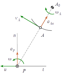
Consider a moving plane with known velocity pole $P$ , rotating with current angular velocity $\\omega$ . For the path of some point $A$ fixed on that plane, we can identify its instant center of curvature $A\_0$ .

These two points are called conjugate points, which are lying together with the velocity pole $P$ on a common line - the pole ray. The velocity $\\bold v\_A$ of point $A$ is directed normal to the pole ray and we get it by

{\\bold v}\_A = {\\bold v}\_P + \\omega\\,{\\tilde \\bold r}\_{PA} \\quad with \\quad \\bold v\_P = \\bold0\\,,

(1)

as the pole has no velocity by definition. The acceleration $\\bold a\_A$ of point $A$ results from derivation of (1) with respect to time

{\\bold a}\_A = {\\bold a}\_P + \\dot\\omega\\,{\\tilde \\bold r}\_{PA} - \\omega^2\\,{\\bold r}\_{PA}\\,,

(2)

with pole acceleration $\\bold a\_P$ and angular acceleration $\\dot\\omega$ of the plane. Dizioglu suggests [7] a rewrite of equation (1) as

{\\bold v}\_A = \\omega\\,{\\tilde \\bold r}\_{PA} = \\omega\\,({\\tilde \\bold r}\_{A}-{\\tilde \\bold r}\_{P})

and deriving it again w.r.t. time yields

{\\bold a}\_A = \\dot\\omega\\,{\\tilde \\bold r}\_{PA} + \\omega\\,{\\dot{\\tilde\\bold r}}\_{A} - \\omega\\,{\\dot{\\tilde\\bold r}}\_{P}\\,.

(3)

Herein is ${\\dot\\bold r}\_{A} = {\\bold v}\_A$ and ${\\dot\\bold r}\_{P}$ is the pole transfer velocity $\\bold u$ . Now comparing components of equations (2) and (3) lets us write the pole transfer velocity in terms of the pole acceleration as

\\bold u = \\frac{{\\tilde \\bold a}\_P}{\\omega}\\,.

(4)

The direction of the pole transfer velocity $\\bold u$ coincides with the direction of the pole tangent $t$ , whereas the pole acceleration $\\bold a\_P$ coincides with the direction of the pole normal $n$ .

We can interprete velocity and normal acceleration of point $A$ additionally to equation (1) as the result of an instantanious rotation about its center of curvature $A\_0$ with angular velocity $\\omega\_A$ , ie.

{\\bold v}\_A = \\omega\_A\\,{\\tilde \\bold r}\_{A\_0A}\\quad and \\quad {\\bold a}\_{A\_n} = -\\omega\_A^2\\,{\\bold r}\_{A\_0A}\\,.

(5)

From these two expressions ${\\bold a}\_{A\_n} = \\omega\_A\\,{\\tilde\\bold v}\_{A}$ can be synthesized and - after multiplying this by ${\\tilde\\bold v}\_{A}$ - we get to

{\\omega}\_A = \\frac{{\\bold a}\_{A\_n}{\\tilde\\bold v}\_{A}}{v\_A^2}\\,.

That term is introduced back into (5), while being allowed to write ${\\bold a}\_{A}{\\tilde\\bold v}\_{A} = {\\bold a}\_{A\_n}{\\tilde\\bold v}\_{A}$ due to the projective character of the dot product. This finally leads us to the location of the center of curvature $A\_0$

{\\bold r}\_{AA\_0} = \\frac{v\_A^2}{{\\bold a}\_{A}{\\tilde\\bold v}\_{A}}{\\tilde\\bold v}\_{A}\\,.

(6)

Equation (1) in its form ${\\bold r}\_{PA} = -\\frac{{\\tilde\\bold v}\_A}{\\omega}$ and (6) can be used for a proof, that in fact points $P$ , $A$ and $A\_0$ are lying on a common line.

Inflection Circle

We now want to have a closer look at points on the moving plane, which are inflection points of their path at current. Those are points at which their curve changes from being concave to convex, or vice versa, so their radius of curvature is instantaniously infinite. Such a point - say $E$ - does not possess normal acceleration, its acceleration $\\bold a\_E$ is rather directed tangential to the curve, as is its velocity $\\bold v\_E$ . So the condition of collinearity between those two has to hold

{\\bold a}\_{E}\\,{\\tilde\\bold v}\_E = 0\\,.

Reusing equations (1) and (2) gives

({\\bold a}\_P + \\dot\\omega\\,{\\tilde \\bold r}\_{PE} - \\omega^2\\,{\\bold r}\_{PE})\\,(-\\omega\\,{\\bold r}\_{PE}) = 0

and resolving the brackets leads to the quadratics

{\\bold r}\_{PE}^2 - \\frac{\\bold a\_P}{\\omega^2}\\bold r\_{PE} = 0\\,.

Completing the square results in

({\\bold r}\_{PE} - \\frac{\\bold a\_P}{2\\omega^2})^2 = \\frac{a\_P^2}{4\\omega^4}\\,,

which has the shape $(\\bold p - \\bold p\_0)^2 = R^2$ of a circle equation in vector notation.

All points on a moving plane, that are inflection points of their path at current, are located on a circle - the inflection circle.

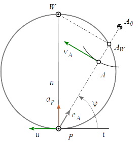
The pole $P$ is also an element of the inflection circle, as it fulfills the above condition due to $\\bold v\_P = \\bold 0$ . The point on this circle opposite to the pole is the inflection pole $W$ (Fig.2). Its location seen from the pole can be extracted as the diameter from the circle equation above as

{\\bold r}\_{PW} = \\frac{\\bold a\_P}{\\omega^2}\\,.

(7)

The Euler-Savary Equation

Substituting ${\\bold r}\_{PA} = -\\frac{{\\tilde\\bold v}\_A}{\\omega}$ from (1) in equation (2) and multiplying that by ${\\tilde\\bold v}\_{A}$ eliminates the term containing the angular acceleration $\\dot\\omega$

{\\bold a}\_A\\,{\\tilde\\bold v}\_{A} = {\\bold a}\_P\\,{\\tilde\\bold v}\_{A} - \\omega\\,v\_A^2\\,.

(8)

Multiplication of equation (6) with ${\\tilde\\bold v}\_{A}$ also yields

{\\bold r}\_{AA\_0}{\\tilde\\bold v}\_{A} = \\frac{v\_A^4}{{\\bold a}\_{A}{\\tilde\\bold v}\_{A}}\\,,

which can be resolved for ${\\bold a}\_{A}{\\tilde\\bold v}\_{A}$ and introduced to (8)

{\\bold a}\_P\\,{\\tilde\\bold v}\_{A} = \\frac{v\_A^4}{{\\bold r}\_{AA\_0}{\\tilde\\bold v}\_{A}} + \\omega\\,v\_A^2\\,.

Now reuse of the terms ${\\tilde\\bold v}\_A = -\\omega\\,{\\bold r}\_{PA}$ and $\\bold a\_P = \\omega^2 {\\bold r}\_{PW}$ from equation (7) helps to remove all kinematic values, finally resulting in the vectorial Euler-Savary equation

{\\bold r}\_{PW}{\\bold r}\_{PA} = r\_{PA}^2\\left(\\frac{r\_{PA}^2}{{\\bold r}\_{AA\_0}{\\bold r}\_{PA}} + 1\\right)\\,.

(9)

The Euler-Savary equation (9) associates conjugate points of a moving plane with the relative location of velocity pole and inflection pole in a pure geometrical form.

The intersection point $A\_W$ of the pole ray with the inflection circle (Fig. 2) is found to be

{\\bold r}\_{PA\_W} = {\\bold r}\_{PA}\\left(\\frac{r\_{PA}^2}{{\\bold r}\_{AA\_0}{\\bold r}\_{PA}} + 1\\right)\\,,

(10)

so Euler-Savary equation can be also written as

{\\bold r}\_{PW}{\\bold r}\_{PA} = {\\bold r}\_{PA} {\\bold r}\_{PA\_W}\\,.

(11)

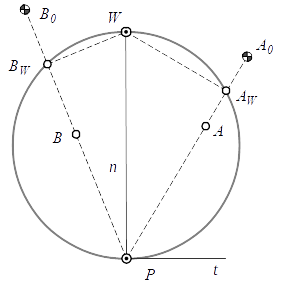
If we happen to know two pairs of conjugate points $A / A\_0$ and $B / B\_0$ on the moving plane, we can determine their intersection points $A\_W$ and $B\_W$ with the inflection circle.

Fig.3: Determination of the Inflection Pole

According to (10) they are

{\\bold r}\_{PA\_W} = {\\bold r}\_{PA}\\left(\\frac{r\_{PA}^2}{{\\bold r}\_{AA\_0}{\\bold r}\_{PA}} + 1\\right)\\quad and \\quad{\\bold r}\_{PB\_W} = {\\bold r}\_{PB}\\left(\\frac{r\_{PB}^2}{{\\bold r}\_{BB\_0}{\\bold r}\_{PB}} + 1\\right)

and with these we are able to write down the Euler-Savary equation two times

{\\bold r}\_{PW}{\\bold r}\_{PA} = {\\bold r}\_{PA} {\\bold r}\_{PA\_W}\\quad and\\quad {\\bold r}\_{PW}{\\bold r}\_{PB} = {\\bold r}\_{PB} {\\bold r}\_{PB\_W}\\,.

Now we can synthesize a geometric vectorial equation for the location of the inflection pole $W$ from those two

{\\bold r}\_{PW} = \\frac{({\\bold r}\_{PB}{\\bold r}\_{PB\_W}){\\tilde\\bold r}\_{PA} - ({\\bold r}\_{PA}{\\bold r}\_{PA\_W}){\\tilde\\bold r}\_{PB}}{{\\tilde\\bold r}\_{PA}{\\bold r}\_{PB}}\\,.

(12)

With the knowledge of two pairs of conjugate points of a moving plane, the location of the reflection pole $W$ can be determined by equation (12).

Equation (12) is a vectorial alternative to Bobillier's construction of the inflection pole.

If we know the inflection pole's location, we can also calculate to any point $A$ on the moving plane its center point $A\_0$ of curvature with the help of Euler-Savary equation (9)

{\\bold r}\_{AA\_0} = \\frac{r\_{PA}^2}{{\\bold r}\_{PW}{\\bold r}\_{PA} - r\_{PA}^2}{\\bold r}\_{PA}\\,.

(13)

Equation (13) is the geometric pendant to kinematic equation (6). When the denominator in (13) becomes zero, the radius of curvature of the path of $A$ is infinite. So the expression

{\\bold r}\_{PW}{\\bold r}\_{PA}- r\_{PA}^2 = 0\\,

is a pure geometric, necessary condition for any point $A$ located on the inflection circle.

The Curvature of Point Paths

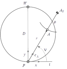
In order to investigate the curvature of the path of a point $A$ of the moving plane in more detail, we align the x-axis of the reference coordinate system with the pole tangent $t$ and the y-axis with the pole normal $n$ .

Fig.4: Notations for discussion of the curvature of a point path

Then we call $\\rho$ the curvature radius, $r$ and $\\psi$ the polar components of the point location $A$ , $r\_0$ the distance from pole $P$ to curvature center $A\_0$ , $\\bold e\_\\psi$ the unit vector from $P$ to $A$ and $D$ the diameter of the inflection circle (Fig. 4).

In this canonical system Euler-Savary equation (9) reads

D\\,r\\,{\\bold e}\_y{\\bold e}\_\\psi = r^2(\\frac{r^2}{\\rho\\,r}+1)\\,.

Using ${\\bold e}\_y{\\bold e}\_\\psi = \\sin\\psi$ we have

D\\sin\\psi = \\frac{r(r+\\rho)}{\\rho}\\,.

(14)

Introducing $r\_0 = r + \\rho$ leads to

D\\sin\\psi = \\frac{r\\,r\_0}{r\_0 - r}\\,,

which - after inverting - results in the well known scalar Euler-Savary equation

\\frac{1}{D} = (\\frac{1}{r} - \\frac{1}{r\_0})\\sin\\psi\\,.

(15)

Herein $r$ and $r\_0$ have to be interpreted as directed quantities. Equation (15) assumes them to be unidirectional. If they have opposite directions, the minus in the parentheses has to be changed to a plus. Using the vectorial form (9), we have the comfort to work with an arbitrary reference coordinate system and don't need to care about signs. Resolving equation (14) for the curvature radius $\\rho$ , yields

\\rho = \\frac{r^2}{D\\sin\\psi - r}\\,,

(16)

which Freudenstein calls the quadratic form of the Euler-Savary equation [8].

The transformation from an arbitrary user coordinate system to the canonical one aligned with pole tangent and pole normal requires the orientation of $\\bold r\_{PW} = D\\,\\bold e\_n\\,$ . By this convention, the x-axis aligned with the pole tangent is directed opposite to the pole transfer velocity $\\bold u\\,$ . A vector from pole $P$ to point $A$ gets transformed into the canonical system and vice versa by pure rotation. Using the matrix

\\bold R(\\varphi\_{n}) = \\begin{pmatrix}-\\tilde\\bold e\_n & \\bold e\_n \\end{pmatrix} = \\begin{pmatrix}\\sin\\varphi\_n & \\cos\\varphi\_n \\\\ -\\cos\\varphi\_n & \\sin\\varphi\_n \\end{pmatrix}

vectors are transformed via

\\bold r\_{PA} = \\bold R(\\varphi\_{n})\\,r\\,\\bold e\_\\psi \\quad and \\quad r \\,\\bold e\_\\psi = \\bold R^T(\\varphi\_{n})\\,\\bold r\_{PA} \\,.

(17)

The Curve of Points of Constant Curvature

All points of a moving plane, possessing the same radius of curvature $\\rho$ of their paths, are located on a curve called $\\rho$ -curve. We get it by resolving equation (16) for $r$

r\_{1,2} = \\frac{\\rho}{2}\\left(-1 \\pm \\sqrt{1+\\frac{4D}{\\rho}\\sin\\psi}\\right)\\,.

(18)

The curve of corresponding centers of curvature results from substituting $r = r\_0 - \\rho$ in equation (16) and resolving for $r\_0$ . Here we yield

r\_{0\_{\\,1,2}} = \\frac{\\rho}{2}\\left(1 \\pm \\sqrt{1+\\frac{4D}{\\rho}\\sin\\psi}\\right)\\,.

(19)

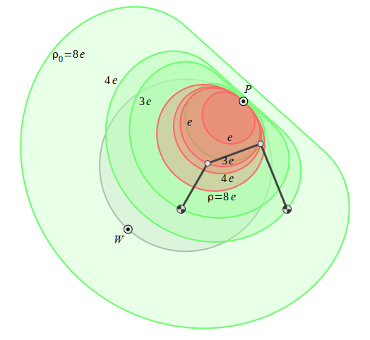
The $\\rho$ Curves and their $\\rho\_0$ pendants of fourbar coupler points with given curvature radii are shown in Fig. 5. Here an abstract length unit $e$ was used. For comparison, both rocker lengths are $3e$ and $4e$ . We can see clearly, that the corresponding curves ( $3e$ and $4e$ ) are running through the coupler joints and their fixed joints respectively.

Fig.5: ρ- and ρ₀-Curves of the Coupler of a Fourbar Mechanism

The plus sign before the square root was used in equations (18) and (19). The alternative curves (negative sign) results in mirrored curves with respect to the pole tangent.

When the given curvature radius goes to infinity, the $\\rho$ -curve approaches the inflection circle.

The Cubic of Stationary Curvature

Some points on the moving plane possess a stationary curvature, i.e. their rate of change of their curvature radius $\\rho$ is zero. In order to get to the cubic of stationary curvature, we need to derive the radius of curvature (16) w.r.t. time and require then

\\frac{d\\rho}{dt} = 0\\,.

As a result we get the cubic curve of centers of stationary curvature. See [1-4, 7-10] for a more indepth discussion.

\\frac{\\sin\\psi\\cos\\psi}{r} = \\frac{\\sin\\psi}{m} + \\frac{\\cos\\psi}{n}

(20)

All we need to know about coefficents $m$ and $n$ is the fact, that they are constant for each particular position of the plane. So, if we can identify two more points on the curve beneath the pole, that have constant curvature for instance - say $A$ and $B$ , we can write down equation (20) two times

\\frac{\\sin\\psi\_A\\cos\\psi\_A}{r\_A} = \\frac{\\sin\\psi\_A}{m} + \\frac{\\cos\\psi\_A}{n}\\quad and\\quad \\frac{\\sin\\psi\_B\\cos\\psi\_B}{r\_B} = \\frac{\\sin\\psi\_B}{m} + \\frac{\\cos\\psi\_B}{n}

and then solve for $m$ and $n$ , which will result in

m = \\frac{r\_A r\_B(\\sin\\psi\_A\\cos\\psi\_B - \\cos\\psi\_A\\sin\\psi\_B)}{\\cos\\psi\_A\\cos\\psi\_B(r\_B\\sin\\psi\_A-r\_A\\sin\\psi\_B)} = \\frac{L^2}{M}

n = \\frac{r\_A r\_B(\\sin\\psi\_A\\cos\\psi\_B - \\cos\\psi\_A\\sin\\psi\_B)}{\\sin\\psi\_A\\sin\\psi\_B(r\_A\\cos\\psi\_B-r\_B\\cos\\psi\_A)} = \\frac{L^2}{N}

Reintroducing those coefficients into (20), while inverting, yields the cubic equation of all points of the moving plane in polar vector notation

r = \\frac{L^2\\sin\\psi\\cos\\psi}{M\\sin\\psi + N\\cos\\psi}\\,.

(21)

Fig.6: The Cubic of Stationary Curvature

The plot of that curve in Fig. 6 shows all points of the fourbar coupler with stationary curvature of their paths. The cubic of stationary curvature belongs to a family of curves mathematically termed strophoids. When the denominator in equation (21) approaches zero, i.e. $M\\sin\\psi + N\\cos\\psi = 0\\,$ , the radial polar component $r$ goes to infinity. From that expression we are able to derive the gradient of the asymptote as

\\tan\\psi\_\\infty = -\\frac{N}{M}\\,.

(22)

With certain poses of the fourbar mechanism one of the constants $M$ or $N$ may reach zero value. In such cases the cubic curve has two branches. One of them is a circle and the other is a straight line. The circle obtained for $N=0$ is then

r = \\frac{L^2}{M}\\cos\\psi\\,.

For plotting the curve in practice, one has to calculate the coordinates $\\bold r = r\\bold\\, e\_\\psi$ with help of equation (21) for a serie of angles $\\psi \\in [0 ... \\pi]$ , or better to avoid the discontinuity at the asymptode $\\psi \\in [\\psi\_\\infty+\\epsilon\\quad ... \\quad\\psi\_\\infty+\\pi-\\epsilon]$ first. Then rotation of the canonical values into the mechanism coordinate system has to be performed by equation (17).

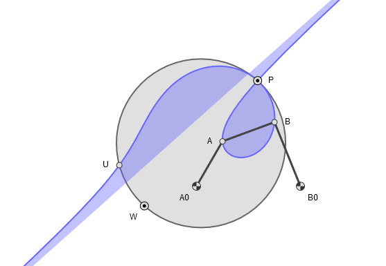
Ball's Point

All points on the cubic possess stationary curvature and all points on the inflection circle are running through an inflection point of their paths, so having instantaneous infinite curvature. Thus the intersection point of the cubic curve with the inflection circle has an important property of stationary infinite curvature of fourth order. That point is called Ball's point and is in fact a point of undulation, where the curvature vanishes, but does not change sign.

The equation of the inflection circle in canonical polar coordinates reads

r = D\\,\\sin\\psi\\,.

Equating it with (21) gives us the angular location of Ball's point $U$

\\tan\\psi\_u = \\frac{L^2-DN}{DM}\\,,

(23)

which has been marked also in Fig. 6.

Conclusion

A discussion of the path curvature of points on a moving plane using a vectorial approach could be done with comparable low effort. The resulting equations prove valuable for practical engineering applications and for visualization via computer graphics.

References

[1] O. Bottema, B. Roth, Theoretical Kinematics, Dover, 1979
[2] R.S. Hartenberg, J. Denavit, Kinematic Synthesis of Linkages, McGraw-Hill, 1964
[3] J.J. Uicker et al., Theory of Machines and Mechanisms. Oxford Press, 2011
[4] M. Husty et al., Kinematik und Robotik. Springer, 1997
[5] S. Gössner, Mechanismentechnik – Vektorielle Analyse ebener Mechanismen, Logos, Berlin, 2016
[6] S. Gössner, Cross Product Considered Harmful.
[7] B. Dizioglu, Getriebelehre - Grundlagen, Vieweg Verlag, 1965.
[8] F. Freundenstein, G. Sandor, Mechanical Design Handbook - Kinematic of Mechanisms, McGraw-Hill, 2006.
[9] W. Blaschke, H.R. Müller, Ebene Kinematik, Oldenbourg Verlasg, 1965.
[10] H. Stachel, Strophoids – Cubic Curves with Remarkable Properties, 24th Symposium on Computer Geometry SCG 2015.