The cross product is frequently used in Physics and Engineering Mechanics. However, the majority of problems in education and practice are planar by nature. Therefore they involve only 2D vectors, while the cross product is limited to 3-space R3.
So, to be a little more specific here:
Cross product is considered harmful with vectors in R2.
As this paper focuses solely on vectors in Euclidean 2-space, we need to discuss possible representations of the cross product in two dimensions.
A well known alternative to vectors are complex numbers. While complex numbers are quite useful to solve planar problems, they cannot be easily generalized to three dimensions. On the contrary, 2D vectors are just a particular case of vectors in R3.
It will be shown below, that coordinate-free vector algebra in R2 can be done completely without the necessity of the cross product, which was introduced by Willard Gibbs in his note
Elements of Vector Analysis around 1880 [8,10,18].
2. Cross Product Matrix in R3
As we intent to eliminate the need for the cross product a closer examination of it in R3 is done first.
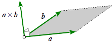
Vector c resulting from the cross product a×b is directed normal to the plane determined by a and
b, so that a, b and c build a right-handed system (Fig.1).
It is obvious, that in 3-space we cannot uniquely define a vector c orthogonal to another vector a. We rather need two linear independent vectors a and b here to get a vector orthogonal to both.
Fig 1: Cross product
The length of c corresponds to the area of the parallelogram spanned by
a and b.
Interestingly there is an alternative pure algebraic approach to the cross product.
Any vector a in R3 can be mapped to a skew-symmetric matrix a~ by partial derivation of the cross product [1]
Now multiplying that matrix with vector b, i.e. a~b yields the same result as the cross product a×b. For that reason this matrix is also termed cross product matrix. The tilde operator, that creates the cross product matrix from any 3D vector, is popular either in kinematics, multi body dynamics and robotics [20,21] as well as in vector graphics [15,25].
2. Orthogonal Operator in R2
So how might that cross product matrix help us with vector space R2 ?
In contrast to 3-space we can find for any single vector in 2-space its unique orthogonal compagnon, as it has to lie in the x/y-plane also. One way to get the orthogonal vector a⊥ to any vector a is utilizing the cross product in combination with unit vector ez normal to x/y-plane
Chace [9] took advantage of this notation for generalizing the solution of planar vector equations in closed-form. Now the cross product matrix in this case can be determined analog to (2)
which looks somewhat like a skew symmetric version of the 2D unit matrix I. If we apply that matrix to vector a its orthogonal vector is obtained. So E is an Orthogonal Operator in R2, which for a proof holds (Ea)(Eb)=ab, which can be easily shown by direct calculation.
The orthogonal operator E, first introduced by Angeles [1-3,10], has interesting properties. Its transposed matrix is equal to its negative matrix (ET=−E) due to skew symmetry. Its determinant is detE=1, so E is not only an orthogonal matrix but also a rotation matrix, rotating any 2D vector by 90° counterclockwise. Multiplication by itself results in the negative unit matrix (E2=−I). The eigenvalues of E are ±i, so we have a direct relationship to the imaginary unit of complex algebra with i2=−1.
With introduction of an orthogonal operator, vectors in R2 have been equipped with a complex structure [19].
Skew symmetric nature of the orthogonal operator is taken
to denote orthogonal 2D vectors by simply writing the ~ symbol over them now, as in
a~=Ea.
So the tilde can be viewed as an orthogonal operator by itself and explicite use of the skew symmetric matrix isn't needed anymore.
Getting the orthogonal 2D vector from another in practice is easy. According to (3) the components simply have to be exchanged while the new first component is negated.
Note that this is different from R3, where a~ is
a skew symmetric matrix. In R2 it is rather the orthogonal vector to a.
This, by the way, corresponds to the fact discussed above, that in order to create an orthogonal vector in R2, a single vector is sufficient, whereas
in R3 two linearly independent vectors are needed.
Use of orthogonal operators, also called perp operator, isn't new of course and can be found documented in [1-4,12,13,16,19,24,25,27]. Interestingly the result of the dot product
a~b=a1b2−a2b1(5)
is identical to the third component of the cross product in (1), which, as a remarkable result, means:
The cross product in particular as well as any explicite outer product in general can be
avoided in vector space R2 by using an orthogonal operator in combination with the dot product instead.
The dot product a~b is a suitable substitute for the cross product in 2-space. Its scalar value is inherited from the cross product and therefore geometrically equivalent to the signed parallelogram area spanned by vectors a and b. This form of the dot product is commonly called perp dot product [16,27], sometimes skew product or due to the latter fact area product [4].
Apart from that, all other known vector rules as commutative, associative and distributive laws will continue to apply.
Regarding the analogy with complex numbers, ab corresponds to the real part
and a~b to the imaginary part of the complex product a∗b, where
a∗ is the complex conjugate of a.
3. Vector Equations in R2
Vector equations can be treated the same as algebraic equations, as they might be added, subtracted and squared. They can be multiplied by a scalar quantity. Multiplication of a vector equation with a vector results in a scalar equation. Multiplying it with a vector again yields a vector equation in turn and so on alternating. Additionally the orthogonal operator can be applied to planar vector equations.
Any vector a and its orthogonal companion a~ are building together an orthogonal basis. An arbitrary other vector might then be expressed as a linear combination of that two
b=λa+μa~.(7)
In order to resolve equation (7) for a the perp operator is applied first
b~=λa~−μa.(8)
Equation (7) is multiplied by λ, equation (8) by μ, then the latter is subtracted from the first
λb−μb~=(λ2+μ2)a
which yields the desired result
a=λ2+μ2λb−μb~.(9)
Equation (7) corresponds to the complex product ab and is therefore representing a similarity transformation. Equation (9) is equivalent to the complex division. Both relations can be shown by direct calculation in coordinate representation.
4. Identities
Any vector c may also be written as a linear combination of two other non-collinear vectors a and b.
c=λa+μb(10)
The scalar coefficients λ and μ with given vectors a, b and c can be resolved through multiplying by b~ and by a~, which elegantly eliminates the respective other term.
λ=−a~bb~candμ=−a~bc~a
Reintroducing the results to (10) and multiplication by common denominator a~b
a(b~c)+b(c~a)+c(a~b)=0,
finally results - after applying the perp operator to that equation - in the Jacobi Identity
Vector space R2 obeys the antisymmetry of its outer product (6) as well as the Jacobi identity (11). By that it
complies with the requirements of being a Lie Algebra [22].
We might proceed in finding identities. An attempt to express the first term in (11) as a linear combination of b and c, i.e.
a~(b~c)=κb+νc
after subsequent multiplication by b~ and c~ respectively yields the scalar coefficients
κ=−ac and ν=ab. Reusing these coefficients in original equation gets us to the Grassmann Identity then.
a~(b~c)=c(ab)−b(ac)(12)
Cyclic commutation of vectors in (12) with abc↦cab and
multiplication by vector d leads to the Binet-Cauchy Identity.
(a~b)(c~d)=(ac)(bd)−(ad)(bc)(13)
For the special case c=a and d=b equation (13) becomes Lagrange's Identity.
(ab)2+(a~b)2=a2b2(14)
5. Polar Vector Representation
Any vector can be decomposed to its length and direction represented by its unit vector.
a=aeαwitheα=(cosαsinα).
This is the polar representation of the vector in 2-space, while α is the angle from the positive x-axis to that vector. It corresponds to the complex polar notation aeiα.
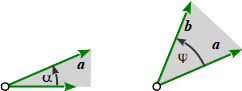
Fig 1: Vector angles
This notation is valuable in geometry and kinematics, as it distinguishable separates lengths and orientations, which may be assigned individual knowns and unknowns then.
Examining the dot product of two vectors
ab=abeαeβ=ab(cosαcosβ+sinαsinβ)
and their perp dot product
a~b=abe~αeβ=ab(cosαsinβ−sinαcosβ),
we get trigonometric expressions for the angle φ=β−α from vector a to vector b after making use of addition theorems of trigonometry
Rotating vector a into vector b by angle φ is achieved via
b=cosφa+sinφa~(16)
which - as a rotation - is a special case of the similarity transformation (7).
6. Time Dependent Vectors
In Kinematics and Multi Body Dynamics we need to deal with time dependent vectors. Here again the polar representation is quite useful, since length and/or orientation of a vector may vary with the time.
Differentiating the direction vector eα with respect to the time gives
where the first summand gives the translational velocity in vector direction and the second summand means the circumferential velocity of the vector rotating with angular velocity α˙.
Further differentiation leads us to the accelerations
Here again the first summand represents the translational/radial component, whereas the second one is the circumferential part including the Coriolis term (second summand in parentheses).
Both velocities (18) and accelarations (19) are variations of the similarity transformation (7) with respect to the orthonormal basis built by eα and e~α.
7. Conclusion
Abandonment of the cross product with planar vectors and simultaneous introduction of an orthogonal operator is a beneficial approach. That small addition to vector operations not only makes an explicite outer product obsolete, but also proves, that vector space R2
is equipped with a complex structure
becomes a Lie Algebra
then. Decomposing a vector a=aeφ in a scalar part and unit vector component, representing length and orientation, is particularly convenient for solving geometric and mechanical problems in a coordinate-free manner, while considerably reducing the amount of trigonometric functions involved.
The proposal to consequently use the orthogonal operator results in a significant improvement for doing vector algebra in R2. This approach has been proven successful in engineering education and practice, as well as computer graphics.
8. References
[1] J. Angeles, The role of the rotation matrix in the teaching of planar kinematics, Mechanism and Machine Theory, 2015.
[2] J. Angeles, R. Sinatra, A novel approach to the teaching of planar mechanism dynamics - a case study, Mechanism and Machine Theory, 2015.
[3] J. Angeles. Fundamentals of Robotic Mechanical Systems: Theory, Methods, and Algorithms. Springer, 2007.
[4] B.B. Bantchev, Calculating with Vectors in Plane Geometry. Mathematics and Education in Mathematics, 2008. Proc. 37th Spring Conf. of the Union of Bulgarian Mathematicians, April 2008, pp.261-267.
[5] O. Bottema, B. Roth, Theoretical Kinematics, Dover, 1979
[6] R.G. Calvet, Treatise of plane geometry through geometric algebra. Eigenverlag, 2007,
[7] J.M. McCarthy et al., Geometric Design of Linkages, Springer, 2010
[8] M.J. Crowe, A History of Vector Analysis, Notre Dame, Indiana, 1967
[9] M. Chace, Vector analysis of linkages, ASME J. Eng. Ind., 1963.
[10] H.R.M. Daniali, Planar Vector Equations in Engineering, Tempus Pub., 2006
[11] J.W. Gibbs, Elements of Vector Analysis, New Haven, 1884
[12] S. Gössner, Analysis of Mechanisms in Vector Space R2, IFToMM D-A-CH conference, Innsbruck, Austria, 2016.
[13] S. Gössner, Mechanismentechnik – Vektorielle Analyse ebener Mechanismen, Logos, Berlin, 2016
[14] R.S. Hartenberg, J. Denavit, Kinematic Synthesis of Linkages, McGraw-Hill, 1964
[15] C. Hecker, Physics, Part 4: The Third Dimension, 2007,
[16] F.S. Hill Jr., The Pleasures of 'Perp Dot' Products, Graphics Gems IV, Academic Press, pp. 138-148, 1994.
[17] M. Husty et al., Kinematik und Robotik. Springer, 1997
[18] P. Lynch, Matthew O'Brian: An Inventor Of Vector Analysis, Irish Math. Soc. Bulletin, 2014
[19] D. Mathews, Complex vector spaces, duals, and duels, 2007.
[20] P.E. Nikravesh, Computer-Aided Analysis of Mechanical Systems. Prentice-Hall, NewJersey, 1988
[21] G. Orzechowski et al., Inertia forces and shape integrals in the floating frame of reference formulation, Springer, 2017.
[22] H. Samelson, Notes on Lie Algebras, 1989.
[23] J.J. Uicker et al., Theory of Machines and Mechanisms. Oxford Press, 2011
[24] VDI-Richtlinie 2120, Vektorrechnung – Grundlagen für die praktische Anwendung, Beuth Berlin, 2005.
[25] J. Vince, Vector Analysis for Computer Graphics, Springer, London, 2007
[26] O. Vinogradov, Fundamentals of Kinematics and Dynamics of Machines and Mechanisms. CRC Press, London, 2000
[27] Wolfram MathWorld, Perp Dot Product,